Connectomics Lab Toolkit

clabtoolkit (Connectomics Lab Toolkit) is a Python toolkit for neuroimaging data processing and analysis, with a focus on brain connectivity, BIDS datasets and common neuroimaging formats.

It is built around a small set of objects (Surface, Parcellation, Tractogram and Connectome) that share a common plotting layer (BrainPlotter), so surfaces, parcellations, streamlines and connectivity matrices can be loaded, processed and visualized with a consistent API. It is designed to work alongside libraries such as nibabel, nilearn and DIPY.

• Free software: Apache Software License 2.0
• Documentation: https://clabtoolkit.readthedocs.io
• Source code: https://github.com/connectomicslab/clabtoolkit

Installation

Install from PyPI:

pip install clabtoolkit

For a development installation:

git clone https://github.com/connectomicslab/clabtoolkit.git
cd clabtoolkit
pip install -e ".[dev]"

Requirements and optional dependencies:

• Python 3.11 or newer.
• 3D plotting (visualizationtools) uses PyVista and needs either a display or off-screen rendering (for example PYVISTA_OFF_SCREEN=true on a server).
• FreeSurfer is not required. The example notebooks retrieve the sample data of clabtoolkit from its Zenodo repository the first time they need it, which needs an internet connection. Only the examples that run FreeSurfer commands, such as annot2gcs, need FreeSurfer.

Features

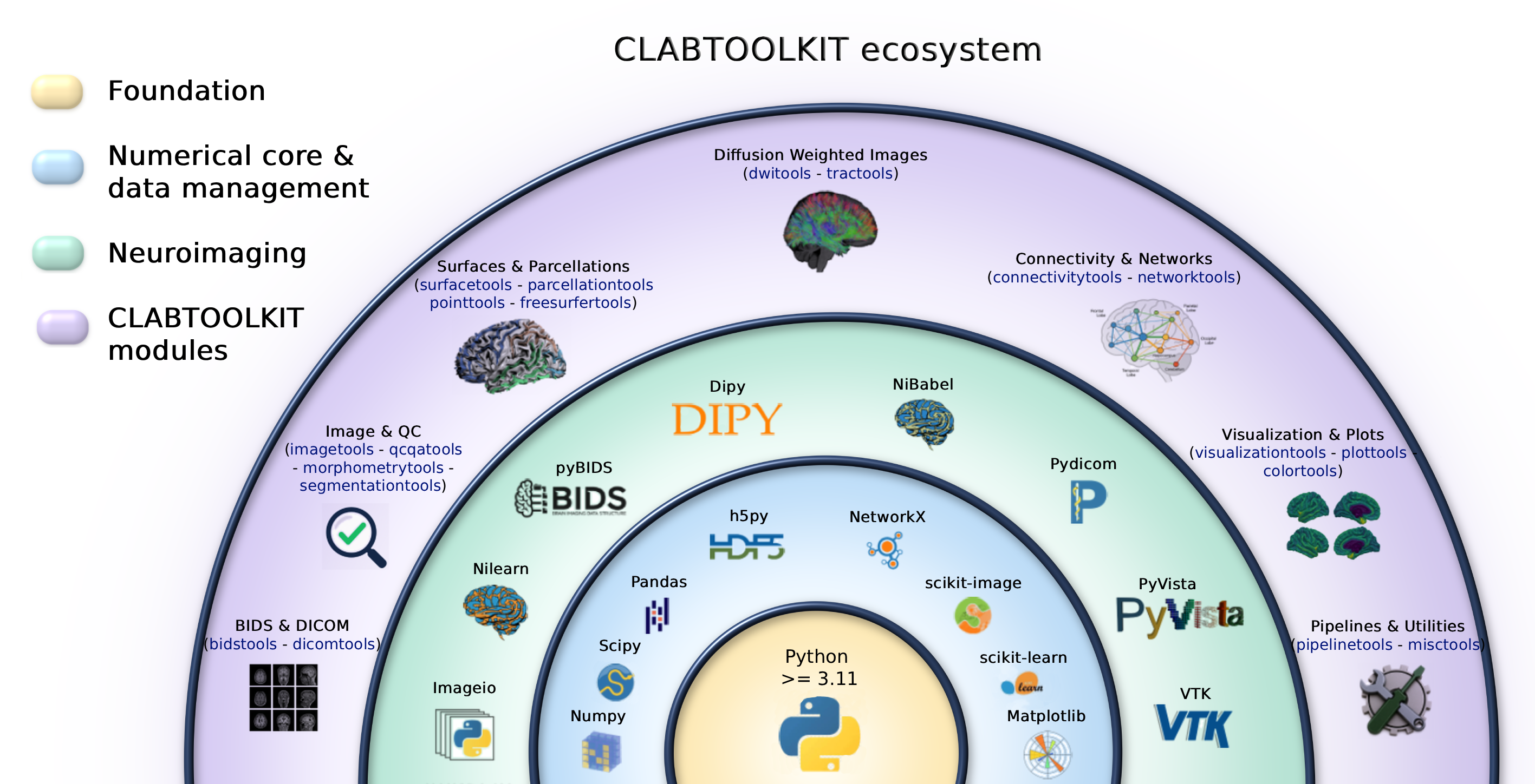
Every module has a notebook with runnable examples in the usage_examples folder (examples-<module>-methods.ipynb), and clabtoolkit_examples.ipynb gives an overview of the whole toolkit.

Data organization

• BIDS Tools (clabtoolkit.bidstools): entity extraction and editing in BIDS filenames, BIDS tree generation and validation, derivatives discovery.
• DICOM Tools (clabtoolkit.dicomtools): DICOM organization, compression and metadata extraction.
• Pipeline Tools (clabtoolkit.pipelinetools): processing-status tables and inventories of derivatives, with JSON and SQLite export.

Images and diffusion

• Image Tools (clabtoolkit.imagetools): voxel/world conversions, cropping, morphology, interpolation, 4D volume handling and image simulation.
• DWI Tools (clabtoolkit.dwitools): volume removal by index or b-value, B0 extraction, acquisition schemes from bvec/bval files, q-space visualization and tensor-derived maps (FA, MD, AD, RD).
• Tract Tools (clabtoolkit.tracttools): the Tractogram class, with streamline filtering, resampling, image interpolation along streamlines, merging and TRK/TCK conversion.
• Segmentation Tools (clabtoolkit.segmentationtools): atlas-based parcellation and tissue segmentation tables.

Surfaces and parcellations

• Surface Tools (clabtoolkit.surfacetools): the Surface class, with scalar maps, annotations, volume-to-surface mapping, smoothing and export.
• Parcellation Tools (clabtoolkit.parcellationtools): the Parcellation class, with region selection by name or code, centroids, volumes, region-wise time series and functional connectivity.
• FreeSurfer Tools (clabtoolkit.freesurfertools): FreeSurfer subjects, annotations, statistics tables and transforms.
• Morphometry Tools (clabtoolkit.morphometrytools): region-wise area, volume and Euler number, and parsing of FreeSurfer statistics.
• Point Tools (clabtoolkit.pointstools): point clouds, merging and curve smoothing.

Connectivity and networks

• Connectivity Tools (clabtoolkit.connectivitytools): the Connectome class, with thresholding, graph metrics, matrix plotting, 3D visualization and CSV/HDF5 I/O.
• Network Tools (clabtoolkit.networktools): sparse-matrix conversion and connected components.

Visualization and utilities

• Visualization Tools (clabtoolkit.visualizationtools): BrainPlotter for surfaces, tractograms and volumes, multi-view layouts and carpet plots.
• Plot Tools (clabtoolkit.plottools): figure layout and font helpers for the plotting classes.
• Colors Tools (clabtoolkit.colorstools): color validation, RGB/hex conversion and color tables.
• Quality Control Tools (clabtoolkit.qcqatools): slice generation and HTML pages for visual quality control.
• Misc Tools (clabtoolkit.misctools): condition-based selection and general-purpose helpers.

What can you do with CLABTOOLKIT?

A few examples of the problems it helps to solve. The full list gives, for each task, the functions that do it and the notebook that shows it.

• Create, convert and export color tables (LUT, TSV, FSL, Nilearn) (ColorTableLoader.load_colortable, ColorTableLoader.export).
• Remove, insert or change BIDS entities in the file names of a whole dataset (recursively_delete_entity, recursively_insert_entity, recursively_replace_entity_value).
• Remove, add and merge regions in a parcellation (Parcellation.remove_by_code, Parcellation.add_parcellation, Parcellation.group_by_codes).
• Compute a morphometry table from a parcellation (Parcellation.compute_morphometry_table).
• Project region values onto surface vertices to create vertex-wise maps and colors (AnnotParcellation.map_values, region_to_vertexwise).
• Load surfaces from several formats and save them back or export them to other formats (Surface.load_from_file, Surface.save_surface).
• Generate structural and functional connectomes directly from a parcellation (Connectome.generate_connectome).
• Create unified morphometry tables, ready for statistical analyses, from FreeSurfer outputs and parcellations (FreeSurferSubject.create_stats_table, create_subject_stats_table).
• Generate slice images and a web page to check the quality of many images quickly (generate_slices, generate_image_selection_webpage).
• Interpolate scalar maps, such as FA, along streamlines (Tractogram.interpolate_on_tractogram).

Quick Start

The examples below use the sample data of clabtoolkit, which is retrieved from its Zenodo repository the first time they run (this needs an internet connection), so you can run them as they are.

Filter a parcellation by region name (keep_by_name)

import clabtoolkit.misctools as cltmisc
import clabtoolkit.parcellationtools as cltparc

# Load the sample parcellation of clabtoolkit (a Chimera parcellation of the Colin27 average brain).
# The color table that is next to the file is found automatically
data_dir = cltmisc.get_sample_data_dir("parcellations")
parc = cltparc.Parcellation(data_dir / "sub-colin27_ses-01_space-tallin_atlas-chimeraDFMFHISIFN_seg-aparc_desc-grow1mm_dseg.nii.gz")

# Keep only the precentral regions (the object is modified in place)
parc.keep_by_name(['ctx-rh-precentral', 'ctx-lh-precentral'])
print(parc.name)  # ['ctx-rh-precentral', 'ctx-lh-precentral']

To load your own parcellation, use cltparc.Parcellation("parc.nii.gz", color_table="lut.txt").

Note

If a file called parc.lut is in the same directory as the parcellation, it is used as the color table by default, so cltparc.Parcellation("parc.nii.gz") is enough. As long as they share the same base name, the LUT file will be automatically detected.

Sample an image along the streamlines of a tractogram (interpolate_on_tractogram)

import clabtoolkit.misctools as cltmisc
import clabtoolkit.tracttools as clttract

# The sample tractogram is retrieved from Zenodo the first time. The sample parcellation is the image
tract_file = cltmisc.get_sample_data_dir("tractograms") / "sub-colin27_ses-01_space-tallin_label-cc_tractogram.trk"
parc_file = cltmisc.get_sample_data_dir("parcellations") / "sub-colin27_ses-01_space-tallin_atlas-chimeraDFMFHISIFN_seg-aparc_desc-grow1mm_dseg.nii.gz"
tract = clttract.Tractogram(tract_file)

# Sample the parcellation at every point of every streamline. The values are labels,
# so the nearest neighbor is used
tract.interpolate_on_tractogram(parc_file, map_name="label",
                                storage_mode="data_per_point", interp_method="nearest")

print(tract.list_maps()["maps_per_point"])  # [..., 'label']
print(tract.data_per_point["label"][0][:5])  # labels along the first streamline

Use interp_method="linear" for scalar images, such as FA, and storage_mode="data_per_streamline" with reduction="mean" to store a single value per streamline.

Plot a surface with a scalar map (BrainPlotter)

import clabtoolkit.misctools as cltmisc
import clabtoolkit.surfacetools as cltsurf
import clabtoolkit.visualizationtools as cltvis

# On a server without a display, set PYVISTA_OFF_SCREEN=true before running

# Load the sample surface and thickness map of clabtoolkit (retrieved from Zenodo the first time)
surf = cltsurf.Surface(cltmisc.get_sample_data_dir("surfaces") / "sub-colin27_ses-01_hemi-L_space-tallin_pial.surf.gii")
surf.load_scalar_maps(cltmisc.get_sample_data_dir("corticalmaps") / "sub-colin27_ses-01_hemi-L_space-tallin_thickness.shape.gii",
                      maps_names="thickness")

# Option 1 (Surface object): plot the lateral and medial views of the map
surf.plot(views=["lateral", "medial"],
          maps="thickness",
          colorbar_title="Thickness (mm)")

# Option 2 (BrainPlotter): the same plot, with more control over colormaps and colorbars
plotter = cltvis.BrainPlotter()
plotter.plot(objs2plot=surf,
             views=["lateral", "medial"],
             map_names="thickness",
             colormaps="hot",
             colorbar=True,
             colorbar_titles="Thickness (mm)")

To plot your own data, load a surface with cltsurf.Surface("lh.pial") and its map with surf.load_scalar_maps("lh.thickness", maps_names="thickness").

Citing

If you use clabtoolkit in your work, please cite the toolkit paper:

Alemán-Gómez, Y., et al. CLABTOOLKIT: An Open-Source Toolkit for Routine Processing, Manipulation, and Visualization of Neuroimaging Data. arXiv:2607.02638. https://arxiv.org/abs/2607.02638

@article{aleman2026clabtoolkit,
  title   = {CLABTOOLKIT: An Open-Source Toolkit for Routine Processing, Manipulation, and Visualization of Neuroimaging Data},
  author  = {Alem{\'a}n-G{\'o}mez, Yasser and Herv{\'e} Nino and Hagmann, Patric},
  journal = {arXiv preprint arXiv:2607.02638},
  year    = {2026},
  url     = {https://arxiv.org/abs/2607.02638}
}

The repository includes a CITATION.cff file, and every release is archived in Zenodo: the DOI 10.5281/zenodo.23540587 always points to the latest version, and each version has its own DOI listed on that page.

Contributing

Contributions are welcome! Please open an issue first to discuss major changes. See CONTRIBUTING.rst for the guidelines, including how to run the test suite.

Changelog

See HISTORY.rst for a detailed changelog.

Credits

Developed by Yasser Alemán-Gómez and collaborators at the Connectomics Lab (Lausanne University Hospital, CHUV). See AUTHORS.rst for the full list.