---

Build interpretable neural networks in PyTorch from a graph of named entities, with checks that every attribution is reported under the right name.

What is kpnn2?

The neurons of a standard neural network have no meaning outside the model. An attribution method can say which neurons a prediction relied on, but not what those neurons stand for.

A knowledge-primed neural network (KPNN) is built from a graph of known entities, such as proteins and the interactions between them, as Figure 1 shows. Every neuron is mapped to one such known entity, and two neurons are connected only when there is a connection between the two entities in the graph (Fortelny and Bock, 2020). The attributions of a KPNN therefore name entities with a domain-meaning, such as proteins, not anonymous neurons.

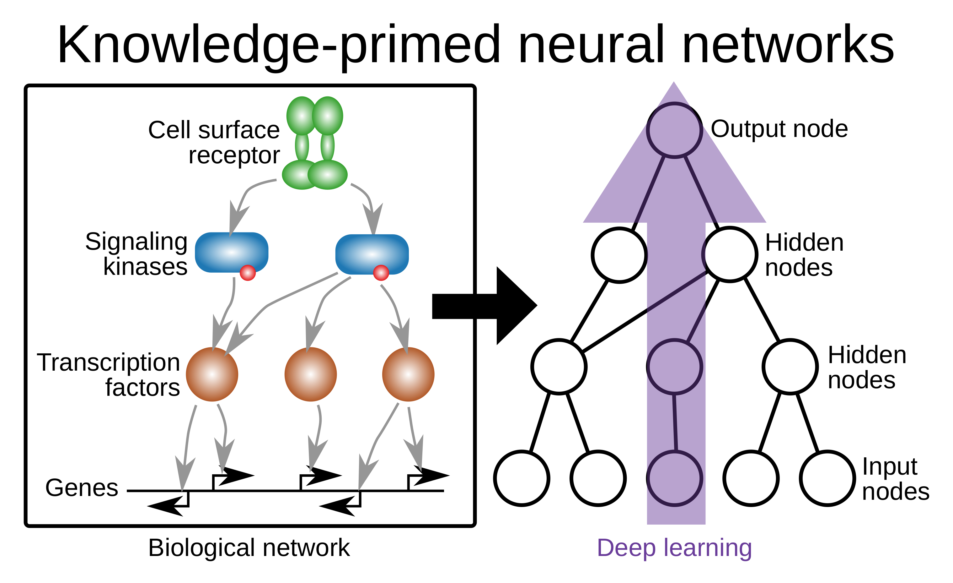
Figure 1. From a network of known protein-protein interactions (and protein-gene interactions) (left) as an example, to a knowledge-primed neural network with the same wiring (right).

kpnn2 builds such networks in PyTorch from an edgelist, which is a table of edges between named entities. kpnn2 in principle can be used in any domain where there are meaningful entities with known relationships between them. When each sample is its own graph, use a graph neural network instead; see Why not a GNN?.

Why kpnn2 exists

The justification of using kpnn2 over custom code is best described with this short story:

"A Scientist's Nightmare: Software Problem Leads to Five Retractions"

In 2006 a structural biology lab retracted five papers, including three papers in Science. An in-house software had swapped two columns of data, which inverted the protein structures the papers reported. Nothing crashed and the results looked plausible. Other labs had based their research on the wrong structures for five years before another group's structure disagreed and revealed the error. (Miller, 2006)

A knowledge-primed neural network has comparable weak spots. Inside PyTorch a protein is only e.g. column 17 of a table of numbers. If your code puts it in the wrong column, or the order changes later, the model still trains and the loss looks normal, but the attributions land on the wrong proteins. kpnn2 aims to prevent that.

Three reasons to use it:

• Checked for correctness. kpnn2 builds the wiring from the edgelist, so you write no masks or indices by hand. It matches input columns by name, refuses a checkpoint with different wiring, and rejects an attribution tensor of the wrong width, among others. Its tests check that only edges in the edgelist can affect a prediction; How we test also lists what is not tested.
• Less code, less to get wrong. In the side-by-side example in Why not custom PyTorch?, one network takes 36 lines with kpnn2 and 162 in hand-written PyTorch, and the hand-written version does not yet align columns, check checkpoints, or label attributions. Every line you do not write is one where a column cannot slip.
• Built on, not rebuilt. kpnn2 provides tested layouts and layers for skip edges, cycles, and attention limited to the graph's edges. This gives you a starting point instead of designing and validating everything on your own, and you can spend your time on the new research question instead.

Why kpnn2 makes the full case and lists every check.

How kpnn2 works

Each row of the edgelist is one edge, from a source node (=neuron) to a target node. Use kpnn2 to parse the edgelist, build the network in PyTorch from the parsing result and train it, then use kpnn2 to label the node attributions derived from the trained network with the right node names (Figure 2). kpnn2 provides building blocks, not a finished model: activations, losses, the training loop, and the attribution method stay your own PyTorch code, which gives you most of the flexibility that PyTorch offers.

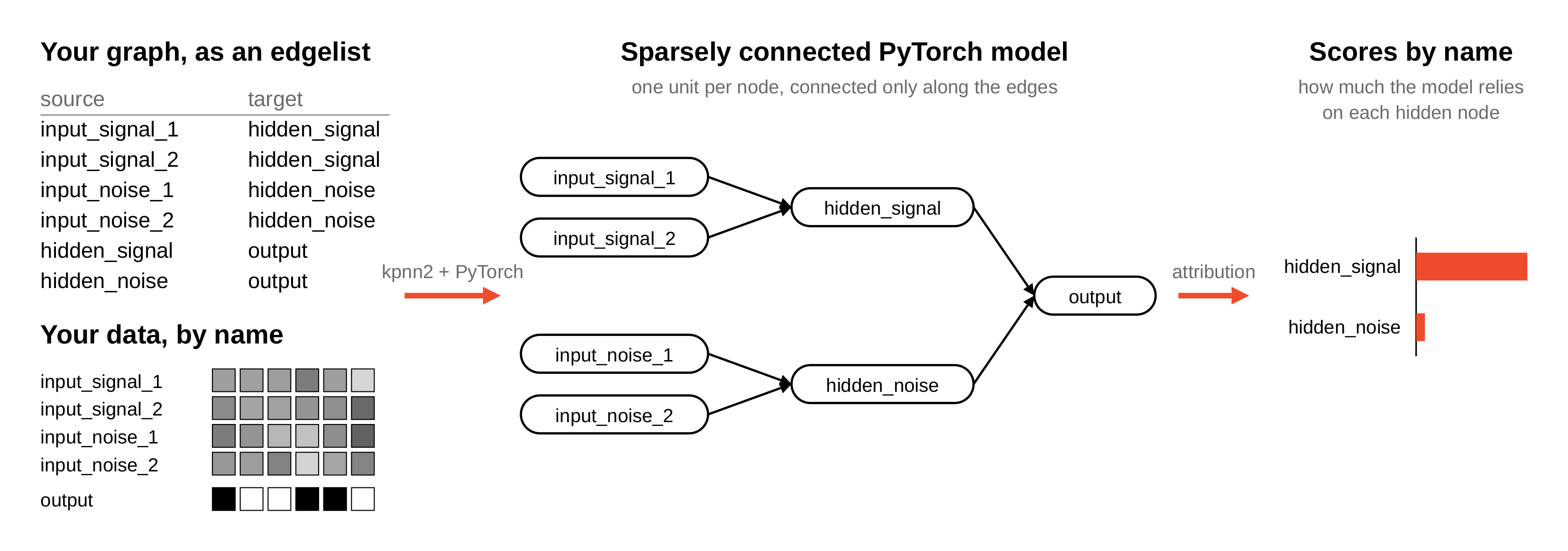
Figure 2. The edgelist, the data, the network, and the attributions all use the same node names. Here the attributions show a model that relies on protein_e in every sample and hardly on protein_f.

The edgelist as the input is either parsed by parse_layered() or by parse_adjacency(), depending on which type of architecture you need (see Supported architectures). By default, parse_layered() places each node in a layer by the longest path that reaches it from an input. An edge that spans more than one layer, such as the dashed edge in Figure 2, is a skip edge. In the edgelist it is one more row, and in the network it gets its own learned weight from the earlier layer: no relay or pseudo neurons are added in between, and it is not a residual connection.

A graph with cycles has no layers, so parse_layered() rejects it. parse_adjacency() accepts cycles and self-loops. It keeps every node in one state vector, and each edge gets its own learned weight between two positions of that vector. Your forward() applies the same connections for as many steps as you choose, so a signal can travel around a cycle. Input nodes have no incoming edges, so you write the inputs into the state vector before each step. If the inputs change at each step, the same update makes a time-series model.

Layered vs. unlayered and the other How it works pages explain how the network is built, and Attributions by node name explains how the attributions get their names.

Installation

Requires Python 3.10 or later.

pip install kpnn2

Quick start

This example builds a model from a small simulated graph, trains it, and reads its attributions by node name. Because the data are simulated, you know in advance which node the model should rely on, and you can check that the attributions agree. The last step uses Captum (pip install captum), which kpnn2 does not depend on.

1. Write the graph as an edgelist

An edgelist has one row per edge, from source to target. parse_layered() sorts the nodes into layers.

import pandas as pd
import torch
from torch import nn

import kpnn2

torch.manual_seed(42)

edgelist = pd.DataFrame(
    [
        ("input_signal_1", "hidden_signal"),
        ("input_signal_2", "hidden_signal"),
        ("input_noise_1", "hidden_noise"),
        ("input_noise_2", "hidden_noise"),
        ("hidden_signal", "output"),
        ("hidden_noise", "output"),
    ],
    columns=["source", "target"],
)
spec = kpnn2.parse_layered(edgelist)
for layer in spec.layer_nodes:
    print(layer)

('input_noise_1', 'input_noise_2', 'input_signal_1', 'input_signal_2')
('hidden_noise', 'hidden_signal')
('output',)

Figure 3 shows this graph, which splits into a signal branch and a noise branch that meet only at output.

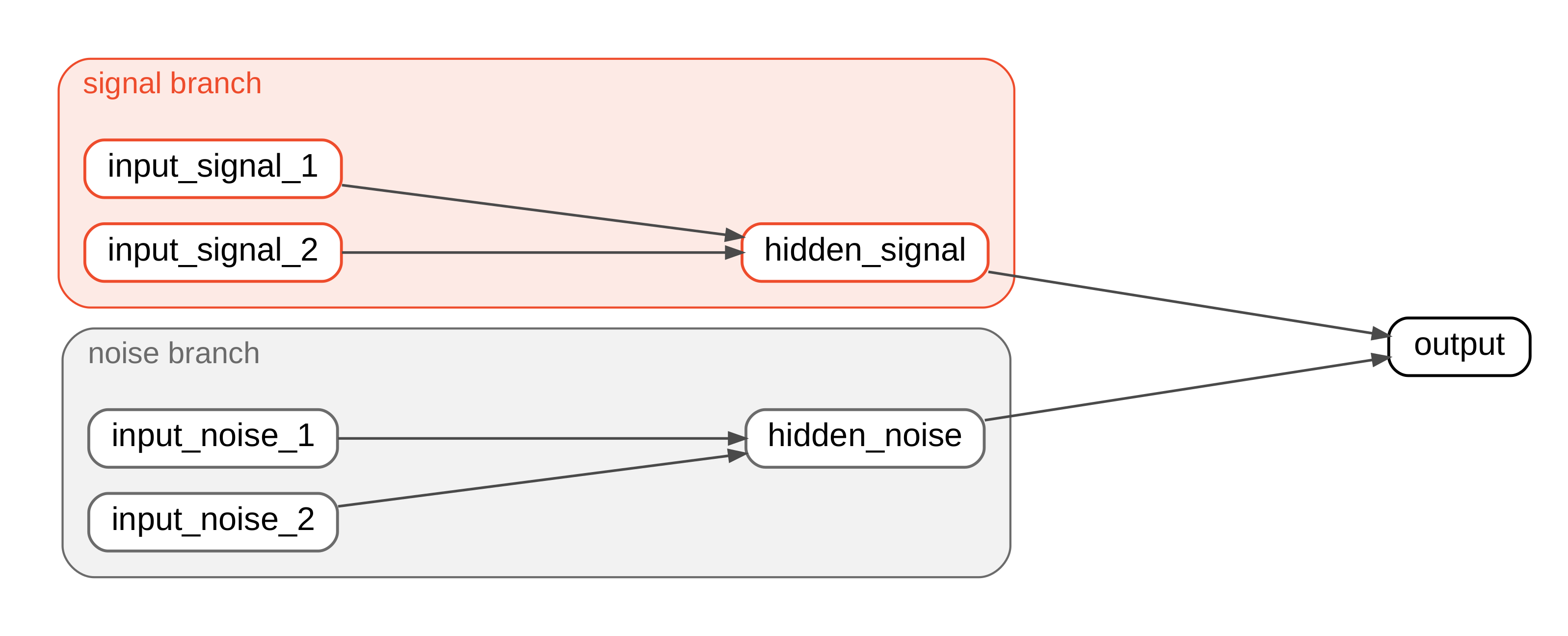
Figure 3. The quick-start graph: inputs on the left, the hidden layer in the middle, and output on the right.

The simulated data are designed so that the signal branch carries information that helps the prediction and the noise branch carries none. A model that learned the task should therefore rely on hidden_signal and give it a high attribution, and give hidden_noise a low one.

2. Build the model in PyTorch

Each hop — the edges entering one layer — becomes one PackedLinear, which stores one weight per edge; PackedLinear.from_hop() builds it from the hop. Without skip edges, each hop reads only the layer before it, so nn.Sequential is enough. With them, a hop also reads earlier layers, and gather_hop_inputs() assembles its input; see Edges that skip layers. identity=spec.fingerprint stores a fingerprint of the graph in each layer. If you later load a checkpoint that was saved from a different graph, the layer raises an error instead of loading weights that belong to other edges.

hop_0, hop_1 = spec.hops
model = nn.Sequential(
    kpnn2.PackedLinear.from_hop(
        hop_0,
        identity=spec.fingerprint,
    ),
    nn.Tanh(),
    kpnn2.PackedLinear.from_hop(
        hop_1,
        identity=spec.fingerprint,
    ),
)

3. Train on data matched by name

align_inputs() puts your feature columns in the order the model expects, by name, so a table in any column order lines up.

input_names = [
    "input_signal_1",
    "input_signal_2",
    "input_noise_1",
    "input_noise_2",
]
features = pd.DataFrame(
    torch.randn(
        200,
        4,
    ).numpy(),
    columns=input_names,
)
labels = features["input_signal_1"] + features["input_signal_2"] > 0

col = kpnn2.align_inputs(
    features.columns,
    spec,
)
x = torch.as_tensor(
    features.to_numpy()[:, col],
    dtype=torch.float32,
)
y = torch.as_tensor(
    labels.to_numpy(),
    dtype=torch.float32,
).unsqueeze(1)

optimizer = torch.optim.Adam(
    model.parameters(),
    lr=0.05,
)
loss_fn = nn.BCEWithLogitsLoss()
for _ in range(200):
    optimizer.zero_grad()
    loss = loss_fn(
        model(x),
        y,
    )
    loss.backward()
    optimizer.step()

4. Read attributions by node name

Run any attribution method on the trained model, then label its output with map_node_attributions(). Here Captum's LayerConductance computes attributions for the hidden layer, and the mean absolute attribution per node summarizes them.

from captum.attr import LayerConductance

conductance = LayerConductance(
    model,
    model[0],
)
attributions = kpnn2.map_node_attributions(
    conductance.attribute(x),
    spec,
    hop_output=hop_0,
)
print(abs(attributions).mean("observation").to_pandas().round(2))

node
hidden_noise     0.39
hidden_signal    4.90
dtype: float32

Figure 4 plots these scores: the trained model relies on hidden_signal and hardly on hidden_noise, so it matches the design of the simulated data which gave only the signal branch helpful information for the prediction.

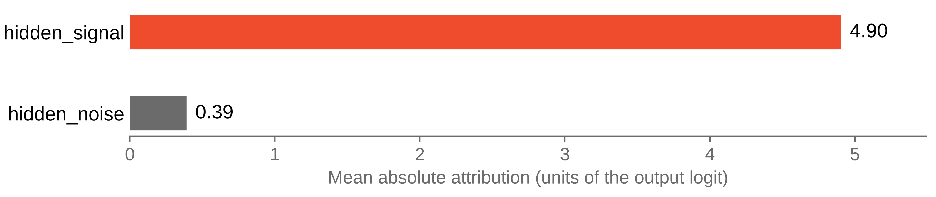
Figure 4. Mean absolute attribution per hidden node in the trained model, from the run above.

The Feedforward example goes further, with a held-out test set, input-level attributions, and a control that moves the signal to the other branch.

Next steps

• Feedforward example for a full tutorial, from edgelist to node-level interpretation
• Supported architectures for cyclic, recurrent, and attention-based models, among others.
• How we test for the tests that pin scientific claims, including a reproduction of a part of Fortelny and Bock (2020)
• API reference for every public name

Citation

If you use kpnn2 in research, please cite the software. Citation metadata is available in CITATION.cff.

License

This project is licensed under the MIT License. See the LICENSE file on GitHub for details.